Blog Viewer

by David A. Swanson, University of California Riverside, Riverside, CA
The Center for Studies in Demography and Ecology, University of Washington, Seattle, WA
Social Science Research Center, Mississippi State University, Starkville, MS                                                                  

Introduction

The US Census Bureau is examining the possibility of creating “synthetic microdata sets” to be used by researchers in place of the “PUMS” (Public Use Microdata Sample) files now being made available. Along with others, I believe that this is a mistake. These synthetic data sets will be created from “real” data by modeling the relationships in the latter and then using the models to generate values in the former. There is a fundamental flaw in this approach: Those attempting to use a synthetic microdata set will have no idea of the relationships in the “real” data underlying the synthetic microdata and the form(s) of the model(s) applied to former to create the latter.

Here, I illustrate this fundamental flaw using a simple, hypothetical example of problems that synthetic data can generate for those using them for research.¹ To set the stage for this example, suppose that you want to set up a website that collects revenue from advertisers based on “hits.” You are told that there is a microdata set from which you can estimate revenue based on hits for the type of website you want to set up. Because of privacy concerns, the microdata set you need to use is comprised of “synthetic data” that shows the number of hits per hour and the amount of revenue generated per hour by the hits (in 100s of dollars), found in Table 1.²

From this hypothetical synthetic microdata set with 11 sets of paired observations, you create a simple regression to show how much revenue you can expect based on hits per hour, as shown in Figure 1.

Figure 1. Estimated Revenue and Hits per Hour Taken from the Synthetic Data Set

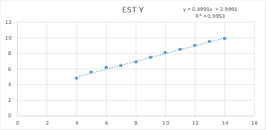
The model has really nice characteristics and you include it as part of your business plan and proceed with your plans to develop the website: expected hourly revenue = 2.9991 + 0.4991*hits, with r² = 0.9953.

Unfortunately, your model may not be as nice as you think. As I show below using four example “real” data sets that could have generated the example synthetic data set, you might have produced very different (and more accurate) models had you been able to work with the real data.

Data Used for the Example

The four data sets are shown in Table 2 represent “Anscombe’s Quartet,” well-known in statistical circles as an illustration of the importance of graphing data prior to analysis (Anscombe, 1973). Under the columns labeled X and Y (the first two columns on the far left) are the X and Y values of Data Set I, where X represents hits and Y represents revenue. To the immediate right are columns that contain the X and Y values for Data Set II. To the right of Data Set II are two columns that contain the X and Y values for Data Set III. Finally, the two rightmost columns contain the X and Y values for Data Set IV.

Each of the four data sets has the same means for X and Y (9.00 and 7.50, respectively) and the same standard deviations (3.32 and 2.03, respectively, for X and Y). All four data sets produce the same regression model, y = 3 + .5*X, r² = 0.67.

 

The Example: In Four Parts

As shown in Figure 2, we see that Data Set I is suitable for building the regression model from which the synthetic data set could have been generated (hourly revenue in $100s ≈ 3 + .5*hourly hits).

Figure 2. Relationship between Revenue and Hits per Hour in Data Set I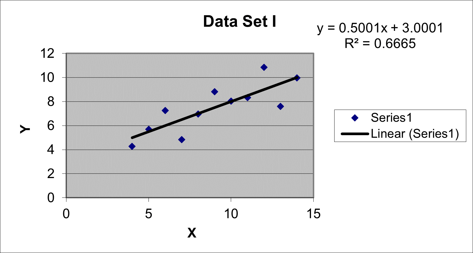

However, Figure 3 shows that, although Data Set II generates the same regression model produced from Data Set I, the relationship between X and Y is decidedly nonlinear. It suggests that, while we could proceed with constructing a regression model to predict values of Y from the values of X, we would likely do better by either “transforming” the data so that they have more of a linear relationship (e.g., by using logarithms) or turning to a more advanced regression technique, one designed to deal with nonlinear relationships between X and Y. In the case of this example, we would not know that the synthetic data set was generated from a simple linear regression instead of a more advanced one that accommodated the nonlinear relationship between X and Y. 

You can see that, if Data Set II represented the “real” data used to generate the synthetic data set, the model we constructed from the synthetic data set would mislead us by indicating that if hits per hour increased steadily, so too would revenue. However, the “real” data show that revenue reaches a peak and then declines as hits per hour increases. Modeling the synthetic data rather than the real data could lead to potentially disastrous decisions for our small business and its expected revenues.

Figure 3. Relationship between Revenue and Hits per Hour in Data Set II

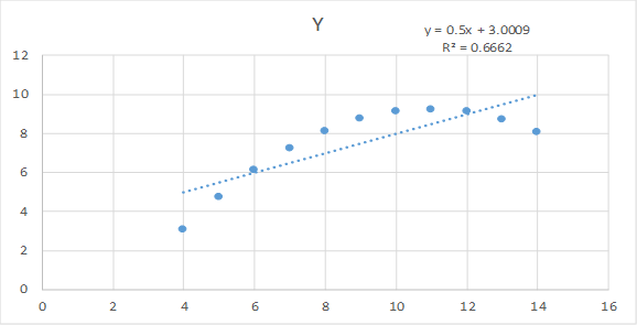
Figure 4 shows that, in Data Set III, the relationship between X and Y is linear but there is an outlier present. This graph suggests that, while we could proceed with constructing a regression model to predict values of Y from the values of X, we would likely do better to deal with the outlier. What users of the synthetic data do not know is that the synthetic data set was generated from the simple linear regression instead of one that dealt with the outlier.

You can see that if Data Set III were the “real” data used to generate the synthetic data set then the model we constructed from the synthetic data set would mislead us by indicating that revenue increases at a higher rate than is the case found in the real data set underlying it. If we had the “real” data, we could remove or modify the outlier and reconstruct the model. For example, by simply removing the outlier, we would have produced a regression model where revenue is not five times the hourly hit rate, but only 4 times the hourly hit rate (estimated revenue in 100s of dollars = .345 +4* hits per hour, r² = 1.00). Again, using the synthetic data could lead to decisions that cause problems for our small business and its expected revenues.

 

Figure 5 indicates that, in Data Set IV, the relationship between X and Y is nonexistent, so a regression model would be an artificial construction made possible by the presence of the outlier. Users of the synthetic data would not know that the synthetic data set was generated from a simple linear regression performed in an inappropriate manner. As is the case with “real” data set II, using a regression model constructed from a synthetic data set based on “real” data set IV would likely lead to disastrous decisions for our small business and its expected revenues (as opposed to the simply problematic decisions based on analyzing synthetic data generated from real data set III).

Figure 5. Relationship between Revenue and Hits per Hour in Data Set IV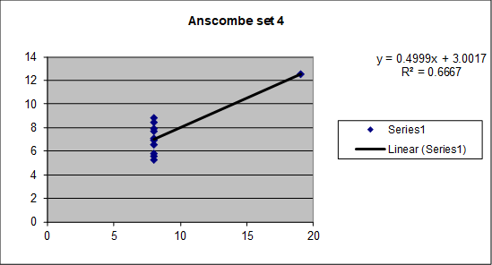

Discussion and Summary

This example shows why you would want to use the “real” data set instead of the synthetic microdata set. Real Data Set I is the only one that could have responsibly generated the synthetic microdata set using a simple regression model. If Data Set II were the real one, a curvilinear model should have been used to construct the synthetic data set, while some outlier modification would have been appropriate had Data Set III been the real data. In the case of Data Set IV, no appropriate model is available to construct synthetic data.

Of course, the Census Bureau will assure us that the synthetic microdata sets it develops will meet all of the standard criteria for the development of models. In the case of the hypothetical example shown here using Anscombe’s Quartet, the Bureau may even go so far as to admit that it was built from a simple linear regression model and met the basic assumptions underlying it. However, even if the Census Bureau went this far, it still means that researchers would have to take a leap of faith. I would be unwilling to take this leap because of the fundamental flaw this simple example reveals in synthetic data: Those attempting to use a synthetic microdata set will have no idea of the relationships in the “real” data underlying the synthetic microdata and the form(s) of the model(s) applied to former to create the latter.

Acknowledgments

I thank Margo Anderson for comments on an earlier draft and Emily Merchant for her editorial assistance.

Endnotes  

1. The Census Bureau creates synthetic data via a modeling process that, while more complicated than the simple examples shown here, are subject to the fundamental problem they illustrate, namely that a researcher knows neither the model(s) used to generate the synthetic data nor the relationships existing among variables in the real data set to which the model(s) were applied. A discussion of the Census Bureau’s use of modeling to create synthetic data is found here.
2. Table 1 was created from Data set I using the regression model that is found from all four data sets in Anscombe’s Quartet, namely (expected revenues in 100s of dollars per hour) = 3 +.5*(hits per hour). Once the regression estimated values were generated they were slightly “jittered” to reflect random results.

Reference

 J. Anscombe (1973). Graphs in Statistical Analysis. The American Statistician 27 (1): 17-21.